Polarization example (GRB) - Stokes parameters method
This notebook fits the polarization fraction and angle of a Data Challenge 3 GRB (GRB 080802386) simulated using MEGAlib and combined with albedo photon background. It’s assumed that the start time, duration, localization, and spectrum of the GRB are already known. The GRB was simulated with 80% polarization at an angle of 90 degrees in the IAU convention, and was 20 degrees off-axis. A detailed description of the Stokes method, which is the approach used here to infer the polarization, is available on the Data Challenge repository.
[1]:
%%capture
from cosipy import UnBinnedData
from cosipy.spacecraftfile import SpacecraftHistory
from cosipy.polarization_fitting.polarization_stokes import PolarizationStokes
from cosipy.threeml.custom_functions import Band_Eflux
from astropy.time import Time
import numpy as np
from astropy.coordinates import Angle, SkyCoord
from astropy import units as u
from scoords import SpacecraftFrame
from cosipy.util import fetch_wasabi_file
from pathlib import Path

%matplotlib inline
Download and read in data
This will download the files needed to run this notebook. If you have already downloaded these files, you can skip this.
Download the unbinned data (660.58 KB), polarization response (1.35 GB), and orientation file (1.10 GB)
[2]:
fetch_wasabi_file('COSI-SMEX/cosipy_tutorials/polarization_fit/grb_background.fits.gz', checksum = '21b1d75891edc6aaf1ff3fe46e91cb49')
fetch_wasabi_file('COSI-SMEX/develop/Data/Responses/ResponseContinuum.o3.pol.e200_10000.b4.p12.relx.s10396905069491.m420.filtered.binnedpolarization.11D.h5', checksum = 'd417d241be0ba7fbfeaef5e2c3bd6ebc')
fetch_wasabi_file('COSI-SMEX/DC4/Data/Orientation/DC4_final_530km_3_month_with_slew_1sbins_GalacticEarth_SAA.fits', checksum = '1b851c042acf4c909798e2401e9d2e38')
A file named grb_background.fits.gz already exists with the specified checksum (21b1d75891edc6aaf1ff3fe46e91cb49). Skipping.
A file named ResponseContinuum.o3.pol.e200_10000.b4.p12.relx.s10396905069491.m420.filtered.binnedpolarization.11D.h5 already exists with the specified checksum (d417d241be0ba7fbfeaef5e2c3bd6ebc). Skipping.
A file named DC4_final_530km_3_month_with_slew_1sbins_GalacticEarth_SAA.fits already exists with the specified checksum (1b851c042acf4c909798e2401e9d2e38). Skipping.
Read in the data (GRB+background) and get the background by reading the files containting background before and after the GRB
[3]:
data_path = Path("") # Update to your path

grb_plus_background = UnBinnedData(data_path/'grb.yaml')
grb_plus_background.select_data_time(unbinned_data=data_path/'grb_background.fits.gz', output_name=data_path/'grb_background_source_interval')
grb_plus_background.select_data_energy(200., 10000., output_name=data_path/'grb_background_source_interval_energy_cut', unbinned_data=data_path/'grb_background_source_interval.fits.gz')
data = grb_plus_background.get_dict_from_fits(data_path/'grb_background_source_interval_energy_cut.fits.gz')
background_before = UnBinnedData(data_path/'background_before.yaml')
background_before.select_data_time(unbinned_data=data_path/'grb_background.fits.gz', output_name=data_path/'background_before')
background_before.select_data_energy(200., 10000., output_name=data_path/'background_before_energy_cut', unbinned_data=data_path/'background_before.fits.gz')
background_1 = background_before.get_dict_from_fits(data_path/'background_before_energy_cut.fits.gz')

background_after = UnBinnedData(data_path/'background_after.yaml') # e.g. background_after.yaml
background_after.select_data_time(unbinned_data=data_path/'grb_background.fits.gz', output_name=data_path/'background_after')
background_after.select_data_energy(200., 10000., output_name=data_path/'background_after_energy_cut', unbinned_data=data_path/'background_after.fits.gz')
background_2 = background_after.get_dict_from_fits(data_path/'background_after_energy_cut.fits.gz')

background = [background_1, background_2]
Read in the response files and the orientation file. Here, the spacecraft is stationary, so we are only using the first attitude bin ( The orientation is cut down to the time interval of the source.)
[4]:
response_file = data_path/'ResponseContinuum.o3.pol.e200_10000.b4.p12.relx.s10396905069491.m420.filtered.binnedpolarization.11D.h5'

sc_orientation = SpacecraftHistory.open(data_path/'DC4_final_530km_3_month_with_slew_1sbins_GalacticEarth_SAA.fits',
                                        tstart = Time(1835493492.2, format = 'unix'), tstop = Time(1835493492.8, format = 'unix')) # e.g. DC4_final_530km_3_month_with_slew_1sbins_GalacticEarth_SAA.fits
Define the GRB spectrum. This is convolved with the response to calculate the ASADs of an unpolarized and 100% polarized source
[5]:
source_direction = SkyCoord(l=23.53, b=-53.44, frame='galactic', unit=u.deg)

a = 100. * u.keV
b = 10000. * u.keV
alpha = -0.7368949
beta = -2.095031
ebreak = 622.389 * u.keV
K = 300. / u.cm / u.cm / u.s

spectrum = Band_Eflux(a = a.value,
                      b = b.value,
                      alpha = alpha,
                      beta = beta,
                      E0 = ebreak.value,
                      K = K.value)

spectrum.a.unit = a.unit
spectrum.b.unit = b.unit
spectrum.E0.unit = ebreak.unit
spectrum.K.unit = K.unit
Define the source position and polarization object
[6]:
asad_bin_edges = Angle(np.linspace(-np.pi, np.pi, 17), unit=u.rad)

source_photons = PolarizationStokes(source_direction, spectrum, asad_bin_edges,
                                    data, sc_orientation, response_file,
                                    background=background, show_plots=False);
Derive the modulation factor. This depends on the source spectrum and the instrument polarization response averaged over polarization angles. This steo needs to be re-computed for every source.
[7]:
average_mu = source_photons._mu100
mu = average_mu['mu']
mu_err = average_mu['uncertainty']

print(f'modulation factor: {mu:.3f} +/- {mu_err:.3f}')
modulation factor: 0.298 +/- 0.000
Derive the minimum detectable polarization, estimated from the source and background spectra and the estimated modulation factor.
[8]:
MDP99 = source_photons._mdp99 * 100
print(f'\nMDP_99: {MDP99:.3f} %')
MDP_99: 16.011 %
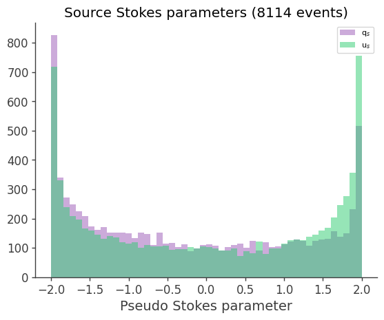
Let’s look at the Pseudo Stokes parameters from the scattering angle for each photon in the data and background simulation
[9]:
source_photons.plot_pseudostokes()
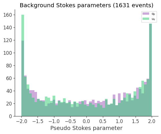
The background is rate is estimated over a longer time period and therefore its flux needs to be rescaled to the expected flux during the GRB. The scale factor is simply the ratio of GRB duration / background duration.
[10]:
print('Background scale factor:', source_photons._backscal)
Background scale factor: 0.0014270214696478288
Fit the polarization of the source from the data.
[11]:
polarization = source_photons.fit(show_plots=True, ref_pdpa=(0.8, 90), ref_label='Simulated');
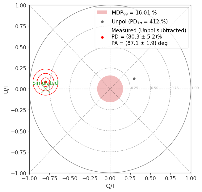
Extracting the information from the polarization dictionary:
[12]:
Pol_frac = polarization['fraction'] * 100
Pol_frac_err = polarization['fraction uncertainty'] * 100
print(f'Polarization degree: ({Pol_frac:.2f} +/- {Pol_frac_err:.2f}) %')

Pol_angle = polarization['angle'].angle.degree
Pol_angle_err = polarization['angle uncertainty'].degree
print(f'Polarization angle: ({Pol_angle:.2f} +/- {Pol_angle_err:.2f}) deg')

Normalized_Q = polarization['QN']
Normalized_U = polarization['UN']
QN_ERR = polarization['QN_ERR']
UN_ERR = polarization['UN_ERR']
print(f'Normalized Q: {Normalized_Q:.3f} +/- {QN_ERR:.3f}')
print(f'Normalized U: {Normalized_U:.3f} +/- {UN_ERR:.3f}')
Polarization degree: (80.34 +/- 5.20) %
Polarization angle: (87.12 +/- 1.88) deg
Normalized Q: -0.799 +/- 0.052
Normalized U: 0.081 +/- 0.053